
Python数据处理学习笔记 - pandas数据合并、重塑和转换篇
这是我阅读《用Python进行数据分析》一书的笔记、实验和总结。本篇文章主要讲解pandas包Series和DataFrame这两大数据结构的以下内容:单个数据集的值检测与处理,多个数据集的合并、重塑、以及包括映射、替换、离散、排列、取样、哑变量等数据转换方法,最后介绍了包括正则在内的对于字符串的处理方法。
第一篇文章主要介绍numpy的ndarray这一多维数组对象,这是Python进行数据分析的基石,也是保证大量数据处理速度的必要条件。第二篇文章主要讲解DataFrame和Series这两个对象本身的使用方法。而本篇文章则着重介绍单个数据集的值检测与处理,多个数据集的合并、重塑、以及包括映射、替换、离散、排列、取样、哑变量等数据转换方法,最后介绍了包括正则在内的对于字符串的处理方法。
对于不同导入格式(CSV、JSON、HDF5、Pickle、Excel、SQL/NoSQL)的导入方法,本文及以后亦不会做详细介绍,请直接翻阅pandas和numpy的I/O部分,所有方法的使用在使用手册中都说明的很详细。其中对JSON的读取效率高于python json模块,但是读取为DataFrame之后,往往不能够很高效的对其进行进一步分析处理,因此还是推荐使用json模块将json对象转化成为Python的字典,然后按需构造DataFrame。至于Excel,pandas使用的是xlrd。如果是大数据集,推荐使用二进制格式,最好是HDF5(适用于多次读一次写)和分块读,效率很高。而频繁写入,最好还是使用SQL/NoSQL数据库。groupby、aggregate、透视、交叉等聚合技术将会在之后逐步介绍。
本文主要内容:从单个数据集导入后的第一步——处理缺失值开始,然后到多个数据集的合并、转置和数据转换。把“单个数据集的值检测和缺失值处理”放在开头而不是和“数据转换”放在一起的原因是,缺失值的优先级很高,并且其属于单个数据集数据剔除、过滤和修剪部分,而不属于数据变换,格式改变等数据转换部分。
约定俗成的,引入numpy、matplotlib和pandas包中DataFrame和Series结构。
import numpy as np
import pandas as pd
PREVIOUS_MAX_ROWS = pd.options.display.max_rows
pd.options.display.max_rows = 20
np.random.seed(12345)
import matplotlib.pyplot as plt
plt.rc('figure', figsize=(10, 6))
np.set_printoptions(precision=4, suppress=True)
%matplotlib inline
1. 单个数据集的值统计和缺失值处理
1.1 存在、唯一和计数
isin([list]) 用来判断存在;unique() 用来生成所有唯一值;value_counts() 用来计数,这个方法也是pandas全局方法,pd.value_counts(obj.values,xxx)
obj = pd.Series(['c', 'a', 'd', 'a', 'a', 'b', 'b', 'c', 'c'])
print(obj.unique().sort()) # 错误,sort不会返回新数据
un = obj.unique();print(un);un.sort();print(un)
None
['c' 'a' 'd' 'b']
['a' 'b' 'c' 'd']
obj.value_counts() #等同于下述
pd.value_counts(obj.values, sort=True)
a    3
c    3
b    2
d    1
dtype: int64
print(obj)
mask = obj.isin(['b', 'c'])
#isin接受一个list作为判断,返回一个bool型索引,
# 可以根据此索引作为切片生成新的数组
print(mask) # 其本质类似于obj[(obj == "b") | (obj == "c")]
print(obj[mask])
print(obj[(obj == "b") | (obj == "c")])
0    c
1    a
2    d
3    a
4    a
5    b
6    b
7    c
8    c
dtype: object
0     True
1    False
2    False
3    False
4    False
5     True
6     True
7     True
8     True
dtype: bool
0    c
5    b
6    b
7    c
8    c
dtype: object
0    c
5    b
6    b
7    c
8    c
dtype: object
value_counts()只适用于Series
>> baby_name.head(3)

	Unnamed: 0	Id	Name	Year	Gender	State	Count
0	11349	11350	Emma	2004	F	AK	62
1	11350	11351	Madison	2004	F	AK	48
2	11351	11352	Hannah	2004	F	AK	46

>> baby_name["Gender"].value_counts()["F"] # Returns 558846
value_count返回所有的value分类结果,而其实我们可以指定返回某些特定值的结果,只需要将这些值的列表转换成index,使用get_indexer来和对象进行比较。【存疑】
to_match = pd.Series(['c', 'a', 'b', 'b', 'c', 'a','e','q'])
unique_vals = pd.Series(['c', 'b', 'a'])
#print(returns.tail())
#print(pd.Index(pd.Series(["0.007846"])).get_indexer(returns.tail()))
print(to_match,unique_vals,pd.Index(unique_vals))
pd.Index(unique_vals).get_indexer(to_match)
#index.get_indexer(obj) 传入一个需要比较的对象,返回这个对象的value和标准index比较后的结果。
                AAPL      GOOG       IBM      MSFT
Date
2016-10-17 -0.000680  0.001837  0.002072 -0.003483
2016-10-18 -0.000681  0.019616 -0.026168  0.007690
2016-10-19 -0.002979  0.007846  0.003583 -0.002255
2016-10-20 -0.000512 -0.005652  0.001719 -0.004867
2016-10-21 -0.003930  0.003011 -0.012474  0.042096

[-1 -1 -1 -1 -1]

0    c
1    a
2    b
3    b
4    c
5    a
6    e
7    q
dtype: object 0
    c

1    b
2    a

dtype: object Index(['c', 'b', 'a'], dtype='object')

array([ 0,  2,  1,  1,  0,  2, -1, -1], dtype=int64)
data = pd.DataFrame({'Qu1': [1, 3, 4, 3, 4],
                     'Qu2': [2, 3, 1, 2, 3],
                     'Qu3': [1, 5, 2, 4, 4]})
data


    Qu1	Qu2	Qu3
    0	1	2	1
    1	3	3	5
    2	4	1	2
    3	3	2	4
    4	4	3	4


result = data.apply(pd.value_counts).fillna(0)
result


        Qu1	Qu2	Qu3
    1	1.0	1.0	1.0
    2	0.0	2.0	1.0
    3	2.0	2.0	0.0
    4	2.0	0.0	2.0
    5	0.0	0.0	1.0
1.2 布尔型索引和数据筛选
对于数据处理来说,bool型索引用作条件对于数据进行清洗是一个非常常见的操作。此部分较为重要,但是因为其并不复杂并且在numpy的ndarray部分已经做过介绍,因此在这里直接略过。
1.3 缺失值处理
缺失值在numpy和pandas中被看作nan,在Python中被看作None,大概有四个方法可以进行缺失值的处理
1.3.1 检测缺失值
检测缺失值需要使用isnull()/isna()/notnull()等函数,一个比较方便的方法,可以快速查看当前列的缺失值情况的是:
df.info() 在这里会看到各个列的索引,还有是否列有缺失值

df.isnull().sum() 可以按照列快速统计缺失值数量。
#需要注意,不能使用df.isnull().count() 这个会统计所有的玩意,包括T和F

#这其实是个谬论,当你越来越了解特殊的、好用的函数,
#你对一个工具了解就越深,但是越容易被束缚,一个通用解决方案是:

for item in df.column:
    getattr(df,item)[getattr(df,item).isnull().any(axis=0)].count()
    #上面这种方法的一个关键在于.any()函数,没有这个参数则不会被过滤。
    #或者 getattr(df,item).isnull().value_counts()[False]
1.3.2 缺失值的丢弃
isnull() or notnull() ; dropna() or fillna()
from numpy import nan as NA
temp = Series([1,23,34,NA,2,31,None]);print(temp)
temp2 = temp.dropna(); #需要注意,dropna()生成一个新的Series。
temp3 = temp[temp.notnull()];print(temp3) #利用boolindex也可以去除缺失值
0     1.0
1    23.0
2    34.0
3     NaN
4     2.0
5    31.0
6     NaN
dtype: float64

0     1.0
1    23.0
2    34.0
4     2.0
5    31.0
dtype: float64
对于DataFrame来说,指定轴axis和how方式可以进行更为细致的处理,比如how="all",axis="index"可以处理全为NA的行。how的值还可以为any
还有一个参数为trash,此参数针对时间序列数据,rows必须包含trash个非NA数据,否则将被去除
temp = DataFrame([[None,None,None,None,None],[None,1,2,3,4],[None,2,3,4,12]]);temp
0	1	2	3	4
0	None	NaN	NaN	NaN	NaN
1	None	1.0	2.0	3.0	4.0
2	None	2.0	3.0	4.0	12.0
print(temp.dropna(axis="index",how="all"))
#temp.dropna(axis=0,how="all")也可以 默认按照行处理
print(temp.dropna(axis=1,how="all"))
print(temp.dropna(how="all").dropna(axis=1))
      0    1    2    3     4
1  None  1.0  2.0  3.0   4.0
2  None  2.0  3.0  4.0  12.0
     1    2    3     4
0  NaN  NaN  NaN   NaN
1  1.0  2.0  3.0   4.0
2  2.0  3.0  4.0  12.0
     1    2    3     4
1  1.0  2.0  3.0   4.0
2  2.0  3.0  4.0  12.0
print(temp.dropna(thresh=5))
print(temp.dropna(thresh=4))
Empty DataFrame
Columns: [0, 1, 2, 3, 4]
Index: []
      0    1    2    3     4
1  None  1.0  2.0  3.0   4.0
2  None  2.0  3.0  4.0  12.0
1.3.3 缺失值的填充
填充缺失数据可以使用fillna() DataFrame.fillna(value=None, method=None, axis=None, inplace=False,limit=None)
传入参数为填充值、填充方法(向前,向后),轴、就地替换,填充多少
frame = DataFrame([[1,2,3],[2,NA,3],[1,NA,NA]]);frame
0	1	2
0	1	2.0	3.0
1	2	NaN	3.0
2	1	NaN	NaN
frame.fillna(0) # 需要注意,不能同时指定 method="ffill"和value,
# 如果指定method,使用limit限制填充数目。
frame.fillna({1:666,2:888}) #不仅仅可以填充标量,还可以填充字典,
# 默认使用column填充不同数值
    0	1	2
0	1	2.0	3.0
1	2	666.0	3.0
2	1	666.0	888.0
frame = DataFrame(np.random.randn(5,5),index=list("12345"),columns=list("abcde"))
frame.iloc[:2,3] = NA;frame.iloc[:4,1]=NA
frame.fillna(method="bfill",limit=3)
    a	b	c	d	e
1	0.373929	NaN 0.230848	1.131250	-0.598619
2	-0.688854	1.356393	2.109390	1.131250	0.293097
3	-0.271625	1.356393	0.549346	1.131250	0.780131
4	0.013845	1.356393	-0.873472	-1.028130	-1.961575
5	-0.302951	1.356393	-0.060635	-1.108226	-0.593790
1.3.4 丢弃指定轴上的项
一般而言,drop可以针对index和column,如果不指定则针对index,如果指定轴为1和指定column是一样的效果。使用inplace可以原地替换。除了drop之外,还可以使用 del df["some column index name"]。
obj = DataFrame(np.random.randint(0,100,size=25).reshape(5,5),
columns=["A","B","C","D","E"]);
print(obj)
newobj = obj.drop(0)
newobj_2 = obj.drop([0,1])
newobj_3 = obj.drop(columns=["D"])
newobj_4 = obj.drop(["E"],axis=1,inplace=True) #可以就地替换
print(newobj,newobj_2,newobj_3,obj,sep="\n\n")
    A   B   C   D   E
0  34  23  41  97  49
1  61  15  78  38  56
2  95   1  91  84   8
3  11  19   1  13  93
4  87  25  96  87  72

    A   B   C   D   E
1  61  15  78  38  56
2  95   1  91  84   8
3  11  19   1  13  93
4  87  25  96  87  72

    A   B   C   D   E
2  95   1  91  84   8
3  11  19   1  13  93
4  87  25  96  87  72

    A   B   C   E
0  34  23  41  49
1  61  15  78  56
2  95   1  91   8
3  11  19   1  93
4  87  25  96  72

    A   B   C   D
0  34  23  41  97
1  61  15  78  38
2  95   1  91  84
3  11  19   1  13
4  87  25  96  87
2. 合并数据
2.0 append: 向DF中添加数据条目
使用append可以快速往一个DF中添加数据:
purchase_1 = pd.Series({'Name': 'Chris',
                        'Item Purchased': 'Dog Food',
                        'Cost': 22.50})
purchase_2 = pd.Series({'Name': 'Kevyn',
                        'Item Purchased': 'Kitty Litter',
                        'Cost': 2.50})
purchase_3 = pd.Series({'Name': 'Vinod',
                        'Item Purchased': 'Bird Seed',
                        'Cost': 5.00})

df = pd.DataFrame([purchase_1, purchase_2, purchase_3], index=['Store 1', 'Store 1', 'Store 2'])

df = df.reset_index()
df = df.set_index(["index","Name"])
df.index.names = ["Location","Name"]
del df["level_0"]

		            Cost	Item    Purchased
Location	Name
Store 1	    Chris	22.5	Dog     Food
            Kevyn	2.5	    Kitty   Litter
Store 2	    Vinod	5.0	    Bird    Seed
DF数据如上,之后使用 append 添加数据,需要注意,对于多Index索引的数据添加,Series需要声明 name 字段,这一字段应该为将要合并后对应的多重index索引元组。
df.append(pd.Series(data={
   "Cost":3.00,
   "Item Purchased":"Kitty Food"},name=("Store 2","Kevyn")))
2.1 merge/join:横轴的合并
使用 pd.merge(on,left_on,right_on,how,copy,suffiex) 进行数据集的合并。
2.1.1 简单轴的合并
需要注意,on如果不指定,则默认按照共同的轴来合并。推荐指定一个轴进行合并
from pandas import DataFrame ,Series
df1 = DataFrame(np.random.randn(10).reshape(5,2),columns=["data","s1"]);
df1["nov"]=[1,2,3,4,5];
df1 = df1.reindex(columns=["nov","data","s1"])

df2 = DataFrame(np.random.randn(10).reshape(5,2),columns=["data","s2"]);
df2["nov"]=[1,2,3,4,5];
df2 = df2.reindex(columns=["nov","data","s2"])
print(df1)
print(df2)
   nov      data        s1
0    1 -0.204708  0.478943
1    2 -0.519439 -0.555730
2    3  1.965781  1.393406
3    4  0.092908  0.281746
4    5  0.769023  1.246435

   nov      data        s2
0    1  1.007189 -1.296221
1    2  0.274992  0.228913
2    3  1.352917  0.886429
3    4 -2.001637 -0.371843
4    5  1.669025 -0.438570
On参数的使用:
pd.merge(df1,df2) #默认会按照所有相同的列来合并
print(pd.merge(df1,df2,on="nov",suffixes=("_1","_2")))
#on可以指定需要参考合并的column,重复的数据会添加_x,_y标签,使用suffixes指定duple。
   nov    data_1        s1    data_2        s2
0    1 -0.204708  0.478943  1.007189 -1.296221
1    2 -0.519439 -0.555730  0.274992  0.228913
2    3  1.965781  1.393406  1.352917  0.886429
3    4  0.092908  0.281746 -2.001637 -0.371843
4    5  0.769023  1.246435  1.669025 -0.438570
how参数的使用:
df1 = df1.loc[:3];print(df1)
df2 = df2.loc[[0,1,2,4]];print(df2)

pd.merge(df1,df2,on="nov",how="inner")
pd.merge(df1,df2,on="nov",how="left").fillna("NA")

print(pd.merge(df1,df2,on="nov",how="outer").fillna("NA"))
//#how的作用是取交集、并集、以左边为准、以右边为准
print(pd.merge(df1,df2,left_on="nov",right_on="nov",how="left").fillna("NA"))
//#其中left_on是指定左边需要比较的column,有时候left_on和
//#right_on不同,需要这样写,而不是使用一个on
   nov      data        s1
0    1 -0.204708  0.478943
1    2 -0.519439 -0.555730
2    3  1.965781  1.393406
3    4  0.092908  0.281746
   nov      data        s2
0    1  1.007189 -1.296221
1    2  0.274992  0.228913
2    3  1.352917  0.886429
4    5  1.669025 -0.438570
   nov     data_x        s1    data_y        s2
0    1  -0.204708  0.478943   1.00719  -1.29622
1    2  -0.519439  -0.55573  0.274992  0.228913
2    3    1.96578   1.39341   1.35292  0.886429
3    4  0.0929079  0.281746        NA        NA
4    5         NA        NA   1.66903  -0.43857
   nov    data_x        s1    data_y        s2
0    1 -0.204708  0.478943   1.00719  -1.29622
1    2 -0.519439 -0.555730  0.274992  0.228913
2    3  1.965781  1.393406   1.35292  0.886429
3    4  0.092908  0.281746        NA        NA
需要注意,left_on和right_on可以传入多行列进行合并。比如,传入:left_on=["column1","column2"] 这样的一个好处是,如果我们需要根据一个人的名字进行合并,对于英文名字(包括姓和名的两个字段),只使用一个字段会导致合并可能出问题,比如James Jobs和James Pocker两个人。因此,可以使用多个字段进行参数传入并且合并。
2.1.2 简单索引的合并
首先构造一个简单索引。
df1["new_index"] = list("aabc");
df1 = df1.set_index("new_index");
df1.index.name = "num";
print(df1)
df2 = DataFrame([23,213,43,12],index=list("accb"),columns=["data"]);
print(df2)
     nov      data        s1
num
a      1 -0.204708  0.478943
a      2 -0.519439 -0.555730
b      3  1.965781  1.393406
c      4  0.092908  0.281746
   data
a    23
c   213
c    43
b    12
简单索引的合并依旧使用merge函数,不过需要声明index参数而不是on参数。
index参数的使用:
print(pd.merge(df1,df2,left_index=True,right_index=True,how="inner"))
#简单索引需要声明left_index和right_index,如果左边的并非索引,而不需要
# 声明left_index,而需要声明left_on
   nov    data_x        s1  data_y
a    1 -0.204708  0.478943      23
a    2 -0.519439 -0.555730      23
b    3  1.965781  1.393406      12
c    4  0.092908  0.281746     213
c    4  0.092908  0.281746      43
2.1.3 层次化索引的合并
和简单索引类似,区别是,如果是column labels和index进行合并,则xx_on需要传递一个包含label name的列表。除此之外,也可以实现index和index的合并。
lefth = pd.DataFrame({'key1': ['Ohio', 'Ohio', 'Ohio',
                               'Nevada', 'Nevada'],
                      'key2': [2000, 2001, 2002, 2001, 2002],
                      'data': np.arange(5.)})
righth = pd.DataFrame(np.arange(12).reshape((6, 2)),
                      index=[['Nevada', 'Nevada', 'Ohio', 'Ohio',
                              'Ohio', 'Ohio'],
                             [2001, 2000, 2000, 2000, 2001, 2002]],
                      columns=['event1', 'event2'])
print(lefth)
print(righth)
   data    key1  key2
0   0.0    Ohio  2000
1   1.0    Ohio  2001
2   2.0    Ohio  2002
3   3.0  Nevada  2001
4   4.0  Nevada  2002
             event1  event2
Nevada 2001       0       1
       2000       2       3
Ohio   2000       4       5
       2000       6       7
       2001       8       9
       2002      10      11
abc = pd.merge(lefth,righth,left_on=["key1","key2"],right_index=True,how="outer")
print(abc)
   data    key1  key2  event1  event2
0   0.0    Ohio  2000     4.0     5.0
0   0.0    Ohio  2000     6.0     7.0
1   1.0    Ohio  2001     8.0     9.0
2   2.0    Ohio  2002    10.0    11.0
3   3.0  Nevada  2001     0.0     1.0
4   4.0  Nevada  2002     NaN     NaN
4   NaN  Nevada  2000     2.0     3.0
left2 = pd.DataFrame([[1., 2.], [3., 4.], [5., 6.]],
                     index=['a', 'c', 'e'],
                     columns=['Ohio', 'Nevada'])
right2 = pd.DataFrame([[7., 8.], [9., 10.], [11., 12.], [13, 14]],
                      index=['b', 'c', 'd', 'e'],
                      columns=['Missouri', 'Alabama'])
abd = pd.merge(left2,right2,left_index=True,right_index=True,how="outer").fillna(0)
print(abd)
   Ohio  Nevada  Missouri  Alabama
a   1.0     2.0       0.0      0.0
b   0.0     0.0       7.0      8.0
c   3.0     4.0       9.0     10.0
d   0.0     0.0      11.0     12.0
e   5.0     6.0      13.0     14.0
join方法
除了使用merge外,其实还可以使用join方法。和merge类似,其也有how、on参数,但是join有lsuffix和rsuffix代替suffixes选项。join可以传入一组DataFrame以连接多个(少用),不过concat也可以。
Join columns with other DataFrame either on index or on a key column
作为比较而言,merge可以连接index和column,更为通用。但是后者可以完全重新制定column名,而不仅仅是添加一个后缀。并且,后者更面向对象一些。
abe = left2.join(right2,how="outer")
print(abe)
   Ohio  Nevada  Missouri  Alabama
a   1.0     2.0       NaN      NaN
b   NaN     NaN       7.0      8.0
c   3.0     4.0       9.0     10.0
d   NaN     NaN      11.0     12.0
e   5.0     6.0      13.0     14.0
2.2 concat:横纵轴的合并
区分与横轴合并使用merge(面向过程)和join(面向对象)方法,Concat连接多用于时间序列等纵轴的合并,虽然concat也是面向过程函数,但是其功能更加强大,可以指定轴,这意味着其也可以完成merge和join的大部分工作。
pandas.concat(objs, axis=0, join='outer', join_axes=None, ignore_index=False, keys=None, levels=None, names=None, verify_integrity=False, copy=True)
参数含义解释:
- axis轴默认为0,也可以设置为1,类似于merge
- join和merge中的how是一个意思
- join_axes是join的高级版,可以更加精细的从纵向选取某些列
- keys可以区分不同数据集的concat,如果axis为1的话,keys即columns。指定keys后会形成多层索引,如果不指定keys,则默认合并相同轴,形成简单索引。
- ignore_index 丢弃连接轴上的索引并生成新的索引
- levels 定义keys在多层索引的级别.
Series的Concat
s1 = pd.Series([0, 1], index=['a', 'b'])
s2 = pd.Series([2, 3, 4], index=['c', 'd', 'e'])
s3 = pd.Series([5, 6], index=['f', 'g'])

print(pd.concat([s1,s2,s3]))
//#一般而言,轴默认为0,如果设置为1,则成为DataFrame。
print(pd.concat([s1,s2,s3],axis=0,join="outer"))
print(pd.concat([s1,s2,s3],axis=0,keys=["A","B","C"]))
print(pd.concat([s1,s2,s3],axis=1))
print(pd.concat([s1,s2,s3],axis=1,join_axes=[["a","c","e"]]))
//#join_axes可以指定选取某些列,其必须为花式索引,axis不能为0.
print(pd.concat([s1,s2,s3],axis=1,keys=["A","B","C"]))
a    0
b    1
c    2
d    3
e    4
f    5
g    6
dtype: int64
a    0
b    1
c    2
d    3
e    4
f    5
g    6
dtype: int64
A  a    0
b    1
B  c    2
d    3
e    4
C  f    5
g    6
dtype: int64
    0    1    2
a  0.0  NaN  NaN
b  1.0  NaN  NaN
c  NaN  2.0  NaN
d  NaN  3.0  NaN
e  NaN  4.0  NaN
f  NaN  NaN  5.0
g  NaN  NaN  6.0
    0    1   2
a  0.0  NaN NaN
c  NaN  2.0 NaN
e  NaN  4.0 NaN
    A    B    C
a  0.0  NaN  NaN
b  1.0  NaN  NaN
c  NaN  2.0  NaN
d  NaN  3.0  NaN
e  NaN  4.0  NaN
f  NaN  NaN  5.0
g  NaN  NaN  6.0
DataFrame的concat
和Series类似,区别是,其默认的join方法为outer,多了一个names参数来定义索引标签名称,如果axis为1,keys为level0的索引。
此外,可以使用ignore_index来丢弃连接轴上的索引并生成新的索引。使用levels指定索引级别。
df1 = pd.DataFrame(np.arange(6).reshape(3, 2), index=['a', 'b', 'c'],
                   columns=['one', 'two'])
df2 = pd.DataFrame(5 + np.arange(4).reshape(2, 2), index=['a', 'c'],
                   columns=['three', 'four'])
print(df1)
print(df2)
   one  two
a    0    1
b    2    3
c    4    5
   three  four
a      5     6
c      7     8
如果不指定axis,默认是纵轴连接,会有四个column,分别是one、two、three和four。而df1和df2的纵轴不会合并。如果指定axis为1,则为横轴连接,也会有四个column,但是纵轴会自动合并,和merge类似。
key参数类似于: fa = pd.concat({"S1":df1,"S2":df2},axis=1,names=["Level0","Level1"]),也可以使用词典key来充当Column Level0 Index Name
level参数类似于:swaplevel("Level0","Level1",axis=1)
print(pd.concat([df1,df2]))
print(pd.concat([df1,df2],axis=0,keys=["A","B"]))
print(pd.concat([df1,df2],axis=1))
print(pd.concat([df1,df2],axis=1,keys=["A","B"]))
four  one  three  two
a   NaN  0.0    NaN  1.0
b   NaN  2.0    NaN  3.0
c   NaN  4.0    NaN  5.0
a   6.0  NaN    5.0  NaN
c   8.0  NaN    7.0  NaN

    four  one  three  two
A   a   NaN  0.0    NaN  1.0
    b   NaN  2.0    NaN  3.0
    c   NaN  4.0    NaN  5.0
B   a   6.0  NaN    5.0  NaN
    c   8.0  NaN    7.0  NaN

one  two  three  four
a    0    1    5.0   6.0
b    2    3    NaN   NaN
c    4    5    7.0   8.0

    A         B
one two three four
a   0   1   5.0  6.0
b   2   3   NaN  NaN
c   4   5   7.0  8.0
2.3 combin_first:重叠数据的合并
一般而言,对于两份几乎一样的数据集,一份作为主要数据集,而这份数据集存在数据缺失,想要从副数据集中提取数据进行填充合并,可以使用 np.where 或者 pandas.combin_first 进行操作。
a = pd.Series([np.nan, 2.5, np.nan, 3.5, 4.5, np.nan],
              index=['f', 'e', 'd', 'c', 'b', 'a'])
b = pd.Series(np.arange(len(a), dtype=np.float64),
              index=['f', 'e', 'd', 'c', 'b', 'a'])
print(a,b)
f    NaN
e    2.5
d    NaN
c    3.5
b    4.5
a    NaN
dtype: float64 f

0.0

e    1.0
d    2.0
c    3.0
b    4.0
a    5.0
dtype: float64
b[-1]=np.nan;b
f    0.0
e    1.0
d    2.0
c    3.0
b    4.0
a    NaN
dtype: float64
np.where(pd.isna(a),b,a) #使用np.where可以自动数据对其并且进行数据合并
array([0. , 2.5, 2. , 3.5, 4.5, nan])
此外,对于pandas来说,可以使用 combine_first
a.combine_first(b) #对于Series,会自动进行数据补齐
f    0.0
e    2.5
d    2.0
c    3.5
b    4.5
a    NaN
dtype: float64
df1 = pd.DataFrame({'a': [1., np.nan, 5., np.nan],
                    'b': [np.nan, 2., np.nan, 6.],
                    'c': range(2, 18, 4)})
df2 = pd.DataFrame({'a': [5., 4., np.nan, 3., 7.],
                    'b': [np.nan, 3., 4., 6., 8.]})
print(df1)
print(df2)
print(df1.combine_first(df2))
//#对于DataFrame而言,会对每个单元格进行修正
     a    b   c
0  1.0  NaN   2
1  NaN  2.0   6
2  5.0  NaN  10
3  NaN  6.0  14

     a    b
0  5.0  NaN
1  4.0  3.0
2  NaN  4.0
3  3.0  6.0
4  7.0  8.0

     a    b     c
0  1.0  NaN   2.0
1  4.0  2.0   6.0
2  5.0  4.0  10.0
3  3.0  6.0  14.0
4  7.0  8.0   NaN
3. 重塑和轴向旋转
3.1 stack堆叠
reshape和pivot。轴向旋转主要使用的函数是stack()和unstack(),以及一个快捷方式:pivote()。
stack和unstack:其中stack可以将列转换成行(也就是生成一个层次化索引的Series)。unstack可以在DataFrame和层次化索引的Series之间进行转换。
data = pd.DataFrame(np.arange(6).reshape((2, 3)),
                    index=pd.Index(['Ohio', 'Colorado'], name='state'),
                    columns=pd.Index(['one', 'two', 'three'],
                    name='number'))
print(data)
number    one  two  three
state
Ohio        0    1      2
Colorado    3    4      5
data.stack()
state     number
Ohio      one       0
          two       1
          three     2
Colorado  one       3
          two       4
          three     5
dtype: int32
print(data.stack().unstack())
number    one  two  three
state
Ohio        0    1      2
Colorado    3    4      5
stack轴选择
stack中有一个关键参数叫做dropna=bool,stack/unstack中的一个关键参数是操作轴,默认而言,是操作最内层进行堆叠,自然,也可以手动指定。
data = pd.DataFrame(np.arange(6).reshape((2, 3)),
                    index=pd.Index(['Ohio', 'Colorado'], name='state'),
                    columns=[["A","B","C"],['one', 'two', 'three']])
data.columns.names = ["Outer","Inner"]
print(data)
Outer      A   B     C
Inner    one two three
state
Ohio       0   1     2
Colorado   3   4     5
print(data.stack("Outer",dropna=False))
print(data.stack("Inner",dropna=True))
Inner           one  three  two
state    Outer
Ohio     A      0.0    NaN  NaN
         B      NaN    NaN  1.0
         C      NaN    2.0  NaN
Colorado A      3.0    NaN  NaN
         B      NaN    NaN  4.0
         C      NaN    5.0  NaN
Outer             A    B    C
state    Inner
Ohio     one    0.0  NaN  NaN
         three  NaN  NaN  2.0
         two    NaN  1.0  NaN
Colorado one    3.0  NaN  NaN
         three  NaN  NaN  5.0
         two    NaN  4.0  NaN
3.2 pivot转换
pivote用于将long/stacked长格式转化成为unstacked宽格式。其实其本质相当于unstack,对stack后的数据使用set_index设置索引,使用unstack进行反向堆叠,然后re_index重新设置索引的过程。
pivote有三个参数,分别是index(按照某个column列作为基准,转换后成为新的row index)、column(某个column列,转换后成为新的column index),value(如果不指定,其余的列会形成符合索引,可以使用re_index设置)。
data = pd.read_csv('examples/macrodata.csv')
print(data.head(3))
     year  quarter   realgdp  realcons  realinv  realgovt  realdpi    cpi  \
0  1959.0      1.0  2710.349    1707.4  286.898   470.045   1886.9  28.98
1  1959.0      2.0  2778.801    1733.7  310.859   481.301   1919.7  29.15
2  1959.0      3.0  2775.488    1751.8  289.226   491.260   1916.4  29.35

      m1  tbilrate  unemp      pop  infl  realint
0  139.7      2.82    5.8  177.146  0.00     0.00
1  141.7      3.08    5.1  177.830  2.34     0.74
2  140.5      3.82    5.3  178.657  2.74     1.09
periods = pd.PeriodIndex(year=data.year, quarter=data.quarter,
                         name='date')
print(periods) #生成一个特殊的Q DEC索引,名称叫做name
columns = pd.Index(['realgdp', 'infl', 'unemp'], name='item')
print(columns) #column索引
PeriodIndex(['1959Q1', '1959Q2', '1959Q3', '1959Q4', '1960Q1', '1960Q2',
             '1960Q3', '1960Q4', '1961Q1', '1961Q2',
             ...
             '2007Q2', '2007Q3', '2007Q4', '2008Q1', '2008Q2', '2008Q3',
             '2008Q4', '2009Q1', '2009Q2', '2009Q3'],
            dtype='period[Q-DEC]', name='date', length=203, freq='Q-DEC')
Index(['realgdp', 'infl', 'unemp'], dtype='object', name='item')
data = data.reindex(columns=columns)
data.index = periods.to_timestamp('D', 'end')
print(data[:4])
ldata = data.stack().reset_index().rename(columns={0:"value"})
print(ldata[:4])
item         realgdp  infl  unemp
date
1959-03-31  2710.349  0.00    5.8
1959-06-30  2778.801  2.34    5.1
1959-09-30  2775.488  2.74    5.3
1959-12-31  2785.204  0.27    5.6
        date     item     value
0 1959-03-31  realgdp  2710.349
1 1959-03-31     infl     0.000
2 1959-03-31    unemp     5.800
3 1959-06-30  realgdp  2778.801
ldata["value2"] = np.random.randn(len(ldata))
print(ldata[:4])
pivot = ldata.pivot(index="date",columns="item",values="value");
pivot2 = ldata.pivot(index="date",columns="item");
print(pivot[:4])
#pivot执行的是和unstack类似的ldata反向操作,需要指定一个index,column的来源。
# 如果含有其余多个列,不指定value的话,则会
#默认生成层次化column索引,否则则抛弃未指定的值。
print(pivot2[:4])
        date     item     value    value2
0 1959-03-31  realgdp  2710.349  0.887204
1 1959-03-31     infl     0.000  0.014331
2 1959-03-31    unemp     5.800 -0.074155
3 1959-06-30  realgdp  2778.801 -0.048565

item        infl   realgdp  unemp
date
1959-03-31  0.00  2710.349    5.8
1959-06-30  2.34  2778.801    5.1
1959-09-30  2.74  2775.488    5.3
1959-12-31  0.27  2785.204    5.6

           value                    value2
item        infl   realgdp unemp      infl   realgdp     unemp
date
1959-03-31  0.00  2710.349   5.8  0.014331  0.887204 -0.074155
1959-06-30  2.34  2778.801   5.1  1.235021 -0.048565 -0.433295
1959-09-30  2.74  2775.488   5.3  0.820211  1.391035 -0.247423
1959-12-31  0.27  2785.204   5.6  0.543980  0.302271 -0.942369
pivot其实就是set_index和unstack的一个快捷方式。对于多余的value2,可以使用层次化索引的reindex进行重新指定。
pivot_like = ldata.set_index(["date","item"]).unstack("item");
pivot_like2 = ldata.set_index(["date","item"]).unstack("item")
.reindex(["value"],level=0,axis=1);

newindex = pd.MultiIndex.from_arrays([["value","value","value","value2","value2"],["infl","unemp","realgdp","unemp","realgdp"]])
print(newindex)

pivot_like3 = ldata.set_index(["date","item"]).unstack("item")
.reindex(newindex,axis=1); #不用写,level=(0,1)了。

pivot_like4 = ldata.set_index(["date","item"]).unstack("item")
.reindex([["value","value","value","value2"],
["infl","unemp","realgdp","unemp"]],axis=1);
#如果声明一个mutipiindex后,不能写,level=(0,1)

print(pivot_like[:3])
print(pivot_like2[:3])
print(pivot_like3[:3])
//#Mutipiindex使用from_array和from_tuple必须在level0级别内分别制定level1的数目
print(pivot_like4[:3])
MultiIndex(levels=[['value', 'value2'], ['infl', 'realgdp', 'unemp']],
           labels=[[0, 0, 0, 1, 1], [0, 2, 1, 2, 1]])

           value                    value2
item        infl   realgdp unemp      infl   realgdp     unemp
date
1959-03-31  0.00  2710.349   5.8  0.014331  0.887204 -0.074155
1959-06-30  2.34  2778.801   5.1  1.235021 -0.048565 -0.433295
1959-09-30  2.74  2775.488   5.3  0.820211  1.391035 -0.247423

           value
item        infl   realgdp unemp
date
1959-03-31  0.00  2710.349   5.8
1959-06-30  2.34  2778.801   5.1
1959-09-30  2.74  2775.488   5.3

           value                    value2
            infl unemp   realgdp     unemp   realgdp
date
1959-03-31  0.00   5.8  2710.349 -0.074155  0.887204
1959-06-30  2.34   5.1  2778.801 -0.433295 -0.048565
1959-09-30  2.74   5.3  2775.488 -0.247423  1.391035

           value                    value2
item        infl unemp   realgdp     unemp
date
1959-03-31  0.00   5.8  2710.349 -0.074155
1959-06-30  2.34   5.1  2778.801 -0.433295
1959-09-30  2.74   5.3  2775.488 -0.247423
arrays = [[1, 1, 2, 2], ['red', 'blue', 'red', 'blue']]
pd.MultiIndex.from_arrays(arrays, names=('number', 'color'))
MultiIndex(levels=[[1, 2], ['blue', 'red']],
           labels=[[0, 0, 1, 1], [1, 0, 1, 0]],
           names=['number', 'color'])
4. 数据剔除、转换和抽取
常见的数据转换主要分为以下几类: 重复数据和缺失值的检测、过滤和替换,map、applymap数据操纵和变换,不同数据形式的转换(离散分组、分类统计、抽样等)。
4.1 值异常:检测和过滤
本质上来说,异常值的过滤是数组运算。一些常用的np函数有any(),abs()和sign()以及describe()。使用bool型索引对其进行过滤。
一个可能的流程是:对于分类数据,可以使用value_counts()和unique()以及isin()进行异常判断;对于连续数据,还可以在此基础上使用describe()和std()(如果我们将大于多少标准差的值看作异常),最后使用bool型索引进行过滤。
需要注意,在过滤数据的时候,DF.any()这个函数很有帮助,bool型索引生成一个ndarray/dataframe,但是是对于每一个元素进行判断的,使用any可以保证对于一行/列,甚至一个level进行判断,如果在这个范围内任意元素出现异常,标记所有行/列/level为异常。然后就可以对其进行过滤。
DataFrame.any(axis=None, bool_only=None, skipna=None, level=None, **kwargs)
data=...
drop data[(np.abs(data)>data.std()*3).any(1)]
# 这个可以对大于三个标准差的数据进行处理
data = pd.DataFrame(np.random.randn(1000, 4))
print(data.describe())
                 0            1            2            3
count  1000.000000  1000.000000  1000.000000  1000.000000
mean      0.042343    -0.044058    -0.029533     0.003557
std       0.990727     0.978300     0.993268     1.025561
min      -3.333767    -2.901831    -3.108915    -3.645860
25%      -0.628630    -0.739475    -0.745047    -0.692099
50%       0.028040    -0.070391    -0.076246     0.028360
75%       0.690847     0.664260     0.634823     0.722198
max       3.525865     2.611678     3.366626     2.763474
data[(np.abs(data) > 3).any(1)] = np.sign(data)*3
print(data.describe())
                 0            1            2            3
count  1000.000000  1000.000000  1000.000000  1000.000000
mean      0.042814    -0.048896    -0.031920     0.008760
std       1.013954     1.015776     1.020521     1.039471
min      -3.000000    -3.000000    -3.000000    -3.000000
25%      -0.654179    -0.751791    -0.748308    -0.694262
50%       0.028040    -0.071723    -0.076246     0.028360
75%       0.713593     0.666408     0.638751     0.725255
max       3.000000     3.000000     3.000000     3.000000
4.3 行列异常:duplicate重复行列移除
duplicate()和drop_duplicate()可以用来查看和删除重复行。其中,如果不指定参数,其默认选取和删除不是第一个的重复值,如果需要反过来,则使用keep="last/first"参数。此外,默认这两者都是根据行的全部列判断重复, 可以传入一个column name的list以用于在这些列判断行是否重复。
data = pd.DataFrame({'k1': ['one', 'two'] * 3 + ['two'],
                     'k2': [1, 1, 2, 3, 3, 4, 4]})
print(data)
    k1  k2
0  one   1
1  two   1
2  one   2
3  two   3
4  one   3
5  two   4
6  two   4
print(data.duplicated())
data.drop_duplicates()
print(data.drop_duplicates(["k2"],keep="last"))
0    False
1    False
2    False
3    False
4    False
5    False
6     True
dtype: bool
    k1  k2
1  two   1
2  one   2
4  one   3
6  two   4
4.3 函数映射转换 map/applymap
映射关系指的是创建一个映射关系列表,然后把元素和一个特定标签或者字符串或者应用函数绑定起来。最常用的映射关系定义一般采用dict,如下:
map = {
    "label1":"value1",
    "label2":"value2"
}
对于元素、行列和索引都可以进行映射,对于值来说,我们用replace函数进行映射替换,对于行列来说,我们用map/applymap进行映射替换,对于索引来说,使用rename进行映射替换。
4.3.1 值处理:replace替换元素
可以使用replace进行替换,第一个参数为需要替换的对象,第二个参数为替换后的对象,可以传递标量和标量、列表和标量、列表和列表,以及字典
data = pd.Series([1., -999., 2., -999., -1000., 3.])
data.replace(-999, np.nan)
0       1.0
1       NaN
2       2.0
3       NaN
4   -1000.0
5       3.0
dtype: float64
data.replace([-999, -1000], np.nan)
0    1.0
1    NaN
2    2.0
3    NaN
4    NaN
5    3.0
dtype: float64
data.replace([-999, -1000], [np.nan, 0])
0    1.0
1    NaN
2    2.0
3    NaN
4    0.0
5    3.0
dtype: float64
data.replace({-999: np.nan, -1000: 0})
0    1.0
1    NaN
2    2.0
3    NaN
4    0.0
5    3.0
dtype: float64
4.3.2 行列处理:map映射
使用map可以将本来已经有的一行/列元素进行替换,也可以创建新的行/列。更灵活的,不仅仅可以使用字典对映射关系进行界定,还可以使用函数,对各个元素进行变换。
data = pd.DataFrame({'food': ['bacon', 'pulled pork', 'bacon',
                              'Pastrami', 'corned beef', 'Bacon',
                              'pastrami', 'honey ham', 'nova lox'],
                     'ounces': [4, 3, 12, 6, 7.5, 8, 3, 5, 6]})
print(data)
          food  ounces
0        bacon     4.0
1  pulled pork     3.0
2        bacon    12.0
3     Pastrami     6.0
4  corned beef     7.5
5        Bacon     8.0
6     pastrami     3.0
7    honey ham     5.0
8     nova lox     6.0
meat_to_animal = {
  'bacon': 'pig',
  'pulled pork': 'pig',
  'pastrami': 'cow',
  'corned beef': 'cow',
  'honey ham': 'pig',
  'nova lox': 'salmon'
}
Series.str.xxx 等同于str.xxx(),对字符串进行的操作。
map可以接受一个函数或者是字典对象,然后生成其对应的序列。
animal = data["food"].str.lower().map(meat_to_animal)
animal = data["food"].map(str.lower).map(meat_to_animal)
#和上述等同,map用来对一连串序列进行函数化操作
animal = data["food"].map(lambda x:meat_to_animal[x.lower()]) #一个更加紧凑的形式
data["animal"] = animal;
print(data)
          food  ounces  animal
0        bacon     4.0     pig
1  pulled pork     3.0     pig
2        bacon    12.0     pig
3     Pastrami     6.0     cow
4  corned beef     7.5     cow
5        Bacon     8.0     pig
6     pastrami     3.0     cow
7    honey ham     5.0     pig
8     nova lox     6.0  salmon
我们也可以同时使用函数和字典,比如这样:
map = {
    "a":"A",
    "b":"B"
}

def myfunc(g):
    return map.get(g,g)

grouped.map(myufunc)

# 同时使用字典和函数可以保证在字典中的映射可以得以改变,而不在字典中的映射则保持原样。
需要注意,map只能够应用于Series/DF的某个Column。对于整个DF进行map需要使用applymap(),或者使用apply指定一个轴。
4.3.3 索引处理:rename重命名
rename可以对所有索引进行更改,可以使用column和index,也可以使用axis。可以传入字典对部分索引更改,使用inplace可以进行原地替换。可以不传入参数,而是传入一个mapper,比如str.upper等。
data = pd.DataFrame(np.arange(12).reshape((3, 4)),
                    index=['Ohio', 'Colorado', 'New York'],
                    columns=['one', 'two', 'three', 'four'])
data.rename({"four":"fff"},axis=1,inplace=False)
#data.rename([["A","B","C"]],axis=1,inplace=False) #不能传递list
# 此外,可以针对index、columns进行参数选择,而不是使用axis,更可以传入一个函数:
print(data.rename(columns=str.upper,inplace=False))
          ONE  TWO  THREE  FOUR
Ohio        0    1      2     3
Colorado    4    5      6     7
New York    8    9     10    11
有时候我们需要将数据的性质进行变换,比如,对于连续型数据,我们需要对其处理以变换成为描述型数据,或者是需要从总体中抽取部分样本做分析,这就需要用到下面的知识:面元划分、计算哑变量和随机抽样。
4.4 离散化和面元划分: (q)cut
对于需要进行分割的数据,使用pd.cut即可。第一个参数为实际数据,第二个参数为分隔段/段数,cut会生成一个categories对象,此对象的codes和categories方法返回原始数据的区分index和categories分段标准本身。一个非常实用的方法是pd.value_counts(categories obj),可以统计在不同段的分别的数值。
cut可以手动传入点列表来分段,也可以自动划分等长的段落,可以指定分段精度以及分段名称,区间闭合选项等。
ages = [20, 22, 25, 27, 21, 23, 37, 31, 61, 45, 41, 32]
bins = [18, 25, 35, 60, 100]
cats = pd.cut(ages, bins,labels=["S","M","L","XL"])
cats
[S, S, S, M, S, ..., M, XL, L, L, M]
Length: 12
Categories (4, object): [S < M < L < XL]
需要注意,cut的第二个参数,可以传递为一个int,表示划分为几份,也可以传递一个list表示按照这些尺度划分。可以传递labels参数以指定这些面元的别称。
print(cats.codes)
print(cats.categories)
pd.value_counts(cats)
closed参数表示开闭。
[0 0 0 1 0 0 2 1 3 2 2 1]
IntervalIndex([(18, 25], (25, 35], (35, 60], (60, 100]]
              closed='right',
              dtype='interval[int64]')

(18, 25]     5
(35, 60]     3
(25, 35]     3
(60, 100]    1
dtype: int64
right参数表示右边包含与否。
pd.cut(ages, [18, 26, 36, 61, 100], right=False) #可以设置左包还是右包。
[[18, 26), [18, 26), [18, 26), [26, 36), [18, 26), ...,
[26, 36), [61, 100), [36, 61), [36, 61), [26, 36)]
Length: 12
Categories (4, interval[int64]):
[[18, 26) < [26, 36) < [36, 61) < [61, 100)]
precision参数指定精度。
data = np.random.rand(20)
pd.cut(data, 5, precision=2) #此外,还可以传递分段数而不是分段点来自动分段
#precision定义精度
[(0.57, 0.76], (0.0027, 0.19], (0.38, 0.57], (0.0027, 0.19], (0.57, 0.76],
..., (0.0027, 0.19], (0.57, 0.76], (0.57, 0.76], (0.0027, 0.19], (0.0027, 0.19]]
Length: 20
Categories (5, interval[float64]):
[(0.0027, 0.19] < (0.19, 0.38] < (0.38, 0.57] < (0.57, 0.76] < (0.76, 0.95]]
qcut()和cut类似,不过其可以保证分段的个数均等,其按照分位数进行分割:
10 for deciles, 4 for quartiles, etc. Alternately array of quantiles, e.g. [0, .25, .5, .75, 1.] for quartiles
data = np.random.randn(1000)  # Normally distributed
cats = pd.qcut(data, 4)  # Cut into quartiles
print(cats)
print(pd.value_counts(cats))
[(0.035, 0.717], (0.035, 0.717], (-0.6, 0.035], (0.717, 3.26], (-0.6, 0.035], ...,
(-3.746, -0.6], (-0.6, 0.035], (0.717, 3.26], (0.035, 0.717], (0.717, 3.26]]
Length: 1000
Categories (4, interval[float64]):
[(-3.746, -0.6] < (-0.6, 0.035] < (0.035, 0.717] < (0.717, 3.26]]
(0.717, 3.26]     250
(0.035, 0.717]    250
(-0.6, 0.035]     250
(-3.746, -0.6]    250
dtype: int64
pd.qcut(data, [0, 0.1, 0.5, 0.9, 1.],precision=2)
[(0.035, 1.32], (0.035, 1.32], (-1.31, 0.035], (0.035, 1.32], (-1.31, 0.035], ...,
(-1.31, 0.035], (-1.31, 0.035], (0.035, 1.32], (0.035, 1.32], (0.035, 1.32]]
Length: 1000
Categories (4, interval[float64]):
[(-3.76, -1.31] < (-1.31, 0.035] < (0.035, 1.32] < (1.32, 3.26]]
4.5 计算指标/哑变量 get_dummies
dummy/indicator variables 叫做指标变量或者哑变量,可以对分类变量使用get_dummies()进行处理。传入一个Series或者DF的某一列,生成一个统计其量值的DataFrame,可以使用join连接原本的列。类似于unstack和value_count的合体。
df = pd.DataFrame({'key': ['b', 'b', 'a', 'c', 'a', 'b'],
                   'data1': range(6)});print(df)
print(pd.get_dummies(df['key']))
   data1 key
0      0   b
1      1   b
2      2   a
3      3   c
4      4   a
5      5   b
   a  b  c
0  0  1  0
1  0  1  0
2  1  0  0
3  0  0  1
4  1  0  0
5  0  1  0
dummies = pd.get_dummies(df['key'], prefix='key')
#prefix为前缀字符串,一般使用指标变量计算时传入Series或者DF的某一列。
print(dummies,type(dummies))
df_with_dummy = df[['data1']].join(dummies) #使用join将一个DF和DF连接起来。
print(df_with_dummy)

# 一个需要注意的点是:
print(type(df[['data1']]),type(df['data1']))
# 使用一般切片切取的是column某一列,其实Series,而是用花式索引切取的是DataFrame。
   key_a  key_b  key_c
0      0      1      0
1      0      1      0
2      1      0      0
3      0      0      1
4      1      0      0
5      0      1      0

<class 'pandas.core.frame.DataFrame'>

   data1  key_a  key_b  key_c
0      0      0      1      0
1      1      0      1      0
2      2      1      0      0
3      3      0      0      1
4      4      1      0      0
5      5      0      1      0

<class 'pandas.core.frame.DataFrame'>

<class 'pandas.core.series.Series'>
mnames = ['movie_id', 'title', 'genres']
movies = pd.read_table('datasets/movielens/movies.dat', sep='::',
                       header=None, names=mnames)
print(movies[:10])
   movie_id                               title                        genres
0         1                    Toy Story (1995)   Animation|Children's|Comedy
1         2                      Jumanji (1995)  Adventure|Children's|Fantasy
2         3             Grumpier Old Men (1995)                Comedy|Romance
3         4            Waiting to Exhale (1995)                  Comedy|Drama
4         5  Father of the Bride Part II (1995)                        Comedy
5         6                         Heat (1995)         Action|Crime|Thriller
6         7                      Sabrina (1995)                Comedy|Romance
7         8                 Tom and Huck (1995)          Adventure|Children's
8         9                 Sudden Death (1995)                        Action
9        10                    GoldenEye (1995)     Action|Adventure|Thriller
all_genres = []
for x in movies.genres:
    all_genres.extend(x.split('|')) #两个list相连使用extend而不是append
genres = pd.unique(all_genres) #使用unique统计唯一值
genres


    array(['Animation', "Children's", 'Comedy', 'Adventure', 'Fantasy',
           'Romance', 'Drama', 'Action', 'Crime', 'Thriller', 'Horror',
           'Sci-Fi', 'Documentary', 'War', 'Musical', 'Mystery', 'Film-Noir',
           'Western'], dtype=object)


```python
zero_matrix = np.zeros((len(movies), len(genres)))
dummies = pd.DataFrame(zero_matrix, columns=genres);
#print(dummies[:10])
gen = movies.genres[0];print(gen)
gen.split('|')
dummies.columns.get_indexer(gen.split('|'))#获取索引所在位置,这里正好是前三个0,1,2
Animation|Children's|Comedy

array([0, 1, 2], dtype=int64)
#第几行就写入第几行的数据,比如i=1,则写入第一行的0,1,2列数据为1
for i, gen in enumerate(movies.genres):
    indices = dummies.columns.get_indexer(gen.split('|'))
    dummies.iloc[i, indices] = 1

movies_windic = movies.join(dummies.add_prefix('Genre_')) #将其统计附加在表的后面
movies_windic.iloc[0][:5]
movie_id                                      1
title                          Toy Story (1995)
genres              Animation|Children's|Comedy
Genre_Animation                               1
Genre_Children's                              1
Name: 0, dtype: object
结合分段的哑变量统计使用非常方便
values = np.random.rand(10)
print(values)
bins = [0, 0.2, 0.4, 0.6, 0.8, 1]
print(pd.cut(values,bins))
print(pd.get_dummies(pd.cut(values, bins).categories))
[0.9296 0.3164 0.1839 0.2046 0.5677 0.5955 0.9645 0.6532 0.7489 0.6536]

[(0.8, 1.0], (0.2, 0.4], (0.0, 0.2], (0.2, 0.4], (0.4, 0.6], (0.4, 0.6],
(0.8, 1.0], (0.6, 0.8], (0.6, 0.8], (0.6, 0.8]]

Categories (5, interval[float64]):
[(0.0, 0.2] < (0.2, 0.4] < (0.4, 0.6] < (0.6, 0.8] < (0.8, 1.0]]

   (0.0, 0.2]  (0.2, 0.4]  (0.4, 0.6]  (0.6, 0.8]  (0.8, 1.0]
0           1           0           0           0           0
1           0           1           0           0           0
2           0           0           1           0           0
3           0           0           0           1           0
4           0           0           0           0           1
4.6 排列和随机取样 sample/permut..
numpy.random.permutation 用于随机化,类似于ramdom.choice().其一是传入标量调用arange(n),其二是传入list,随机list的元素值.
此外,还可以使用simple(n,widght,axis)来直接从Series或者DataFrame进行取样
np.random.permutation(10)
array([1, 3, 9, 6, 5, 0, 4, 2, 7, 8])
np.random.permutation(["A","B","C","D","E","F","G"])
array(['B', 'F', 'E', 'C', 'G', 'D', 'A'], dtype='<U1')
df = pd.DataFrame(np.arange(5 * 4).reshape((5, 4)))
print(df)
df.take(np.random.permutation(5)[:3],axis=0).take(np.random.permutation(4),axis=1)
#随机化轴的索引顺序,
#Return the elements in the given positional indices along an axis.
#在随机化轴顺序时take还可以限制只取一部分样
    0   1   2   3
0   0   1   2   3
1   4   5   6   7
2   8   9  10  11
3  12  13  14  15
4  16  17  18  19
print(df.sample(n=3,axis=0).sample(n=3,axis=1))
print(df.sample(n=3,axis=0).sample(frac=0.5,axis=1))
#此外,还可以按照比率进行取值而不仅仅是指定数目大小,n和frac不能同时使用。
    1   3   0
0   1   3   0
3  13  15  12
4  17  19  16

    3   2
3  15  14
2  11  10
1   7   6
4.7 数据尺度和类型转换
常见的数据尺度有四种:分类的、有序的、等距的和等比的。 一般我们需要对于分类和后者进行区分。
在DF/S中,我们可以定义一个有序序列数据,这样的好处显而易见,可以进行大小比较,使用max、min等函数。
s = pd.Series(['Low', 'Low', 'High', 'Medium',
'Low', 'High', 'Low'])

s.astype("category",categories=["Low","Medium","High"],ordered=True)
如上所示,直接对Series使用astype,传入“category”这一数据类型,设置其来源池,这样就构造了分类数据,任何不在分类数据池中的数据会被标记为NaN。如果传入ordered参数为True就是有序数据,左边小,右边大。
5. 字符串处理
5.1 Python原生字符串处理方法
val = 'a,b,  guido'
val.split(',')
pieces = [x.strip() for x in val.split(',')]
pieces
first, second, third = pieces
first + '::' + second + '::' + third
'::'.join(pieces)
'guido' in val
val.index(',')
val.find(':')
val.index(':')
val.count(',')
val.replace(',', '::')
val.replace(',', '')
5.2 Python正则表达式
Python正则表达式需要使用 regex=re.compile("rules") 先创建一个规则,然后使用findall寻找所有匹配,使用match匹配开头,使用search匹配一个,使用split进行分割,使用sub进行替换。
import re
regex = re.compile('\s+')
regex.split("foo bar baz \nqux")
['foo', 'bar', 'baz', 'qux']
regex.findall("foo bar baz \nqux")
[' ', ' ', ' \n']
text = """Dave dave@google.com
Steve steve@gmail.com
Rob rob@gmail.com
Ryan ryan@yahoo.com
"""
pattern = r'[A-Z0-9._%+-]+@[A-Z0-9.-]+\.[A-Z]{2,4}'

# re.IGNORECASE makes the regex case-insensitive
regex = re.compile(pattern, flags=re.IGNORECASE)
regex.findall(text)
['dave@google.com', 'steve@gmail.com', 'rob@gmail.com', 'ryan@yahoo.com']
m = regex.search(text)
m
text[m.start():m.end()]
'dave@google.com'
print(regex.match(text))
print(regex.sub('REDACTED', text))
pattern = r'([A-Z0-9._%+-]+)@([A-Z0-9.-]+)\.([A-Z]{2,4})'
regex = re.compile(pattern, flags=re.IGNORECASE)
m = regex.match('wesm@bright.net')
m.groups()
regex.findall(text)
print(regex.sub(r'Username: \1, Domain: \2, Suffix: \3', text))
5.3 矢量化字符串处理方法
按理来说,可以直接使用正则和Python自带的字符串方法对多维数组进行操作,但是一个问题是NaN的问题,map函数会出错,因此DataFrame.str内置了很多字符串处理方法。
比如普通Python字符串的in方法(使用contains),正则表达式的findall和match。
data = {'Dave': 'dave@google.com', 'Steve': 'steve@gmail.com',
        'Rob': 'rob@gmail.com', 'Wes': np.nan}
data = pd.Series(data)
print(data)
data.isnull()
Dave     dave@google.com
Rob        rob@gmail.com
Steve    steve@gmail.com
Wes                  NaN
dtype: object


Dave     False
Rob      False
Steve    False
Wes       True
dtype: bool
data.str.contains('gmail')
Dave     False
Rob       True
Steve     True
Wes        NaN
dtype: object
pattern
data.str.findall(pattern, flags=re.IGNORECASE)
Dave     [dave@google.com]
Rob        [rob@gmail.com]
Steve    [steve@gmail.com]
Wes                    NaN
dtype: object
matches = data.str.match(pattern, flags=re.IGNORECASE) #对各个元素执行re.match。
matches
Dave     True
Rob      True
Steve    True
Wes       NaN
dtype: object
data.str[:5] #此外,str还支持slice、split、replace、strip等常用字符串方法。
Dave     dave@
Rob      rob@g
Steve    steve
Wes        NaN
dtype: object
6. 时间序列处理
这里只提一下DatetimeIndex索引和PeriodIndex这个索引,在时间序列中经常看到。
class pandas.DatetimeIndex 一个很有用的方法:
- DatetimeIndex.to_period(freq=None) 可以在datetimeindex和periodindex进行转换,freq可以为A、M、D,表示按照年、月、日聚合
class pandas.Period 有两个很方便的方法:
- asfreq(M) # 格式转换,同上
- strftime(format like "%m%d") 转换成字符串
还有一个函数,叫做period_range,可以生成一个PeridIndex,它的作用是可以在PeriodIndex构成的DataFrame中快速选择某一部分数据。
pandas.period_range(start=None, end=None, periods=None, freq='D', name=None)
pd.period_range(start='2017-01-01', end='2018-01-01', freq='M')
PeriodIndex(['2017-01', '2017-02', '2017-03', '2017-04', '2017-05',
         '2017-06', '2017-06', '2017-07', '2017-08', '2017-09',
         '2017-10', '2017-11', '2017-12', '2018-01'],
        dtype='period[M]', freq='M')

pd.period_range(start=pd.Period('2017Q1', freq='Q'),
           end=pd.Period('2017Q2', freq='Q'), freq='M')
PeriodIndex(['2017-03', '2017-04', '2017-05', '2017-06'],
            dtype='period[M]', freq='M')
最后顺便提一下,如何将object格式的index转化成PeriodIndex:
- df.columns = df.columns.to_period(freq) #Series.to_period(freq=None, copy=True)
- df.columns = df.columns.astype('datetime64[ns]').to_period(freq="D")
7. 示例:USDA食品数据库.json
data = pd.read_json("datasets/usda_food/database.json");
index = ["description","group","id","manufacturer"]
info = DataFrame(data,columns=index);
print(info[:5])
                          description                   group    id  \
0                     Cheese, caraway  Dairy and Egg Products  1008
1                     Cheese, cheddar  Dairy and Egg Products  1009
2                        Cheese, edam  Dairy and Egg Products  1018
3                        Cheese, feta  Dairy and Egg Products  1019
4  Cheese, mozzarella, part skim milk  Dairy and Egg Products  1028

  manufacturer
0
1
2
3
4
info.group.value_counts()
Vegetables and Vegetable Products    812
Beef Products                        618
Baked Products                       496
Breakfast Cereals                    403
Legumes and Legume Products          365
Fast Foods                           365
Lamb, Veal, and Game Products        345
Sweets                               341
Fruits and Fruit Juices              328
Pork Products                        328
                                    ...
Ethnic Foods                         165
Snacks                               162
Nut and Seed Products                128
Poultry Products                     116
Sausages and Luncheon Meats          111
Dairy and Egg Products               107
Fats and Oils                         97
Meals, Entrees, and Sidedishes        57
Restaurant Foods                      51
Spices and Herbs                      41
Name: group, Length: 25, dtype: int64
import json
ndata = json.loads(open("datasets/usda_food/database.json").read())
nutrients = ndata[0]["nutrients"];
nutrients = DataFrame(nutrients)
print(nutrients.head(5))
                   description        group units   value
0                      Protein  Composition     g   25.18
1            Total lipid (fat)  Composition     g   29.20
2  Carbohydrate, by difference  Composition     g    3.06
3                          Ash        Other     g    3.28
4                       Energy       Energy  kcal  376.00
print(nutrients.duplicated().sum())
a = nutrients.drop_duplicates()
108
nindex = ["description","group","id","manufacturer"]
info = DataFrame(ndata,columns=nindex);
print(info.head())
                          description                   group    id  \
0                     Cheese, caraway  Dairy and Egg Products  1008
1                     Cheese, cheddar  Dairy and Egg Products  1009
2                        Cheese, edam  Dairy and Egg Products  1018
3                        Cheese, feta  Dairy and Egg Products  1019
4  Cheese, mozzarella, part skim milk  Dairy and Egg Products  1028

  manufacturer
0
1
2
3
4
nutrients = []
for item in ndata:
    itemdf = DataFrame(item["nutrients"])
    itemdf["id"] = item["id"]
    nutrients.append(itemdf)
nutrients = pd.concat(nutrients,ignore_index=True)
nutrients = nutrients.rename({"group":"nutgroup","description":"nutrient"},copy=False,axis=1)
info = info.rename({"group":"fgroup","description":"food"},copy=False,axis=1)
ndata = pd.merge(info,nutrients,on="id",how="outer")
print(ndata.head())
              food                  fgroup    id manufacturer  \
0  Cheese, caraway  Dairy and Egg Products  1008
1  Cheese, caraway  Dairy and Egg Products  1008
2  Cheese, caraway  Dairy and Egg Products  1008
3  Cheese, caraway  Dairy and Egg Products  1008
4  Cheese, caraway  Dairy and Egg Products  1008

                      nutrient     nutgroup units   value
0                      Protein  Composition     g   25.18
1            Total lipid (fat)  Composition     g   29.20
2  Carbohydrate, by difference  Composition     g    3.06
3                          Ash        Other     g    3.28
4                       Energy       Energy  kcal  376.00
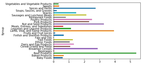
result = ndata.groupby(["nutrient","fgroup"])["value"].quantile(0.5)
result
nutrient          fgroup
Adjusted Protein  Sweets                               12.900
                  Vegetables and Vegetable Products     2.180
Alanine           Baby Foods                            0.107
                  Baked Products                        0.248
                  Beef Products                         1.550
                  Beverages                             0.003
                  Breakfast Cereals                     0.311
                  Cereal Grains and Pasta               0.373
                  Dairy and Egg Products                0.273
                  Ethnic Foods                          1.290
                                                        ...
Zinc, Zn          Nut and Seed Products                 3.290
                  Pork Products                         2.320
                  Poultry Products                      2.500
                  Restaurant Foods                      0.800
                  Sausages and Luncheon Meats           2.130
                  Snacks                                1.470
                  Soups, Sauces, and Gravies            0.200
                  Spices and Herbs                      2.750
                  Sweets                                0.360
                  Vegetables and Vegetable Products     0.330
Name: value, Length: 2246, dtype: float64
result["Zinc, Zn"].plot(kind="barh")
<matplotlib.axes._subplots.AxesSubplot at 0x4912cc5cf8>
————————————————————————————————————
更新日志
2018-02-27 完成《利用Python进行数据分析》阅读和笔记
2018-03-25 完成笔记补充和目录整理
2018-03-28 na值处理的笔记补充,添加了StringIO读写的说明。
2018-04-25 添加了布尔型索引筛选数据部分,添加了append合并数据部分。
2018-05-12 添加时间序列处理